Ability to Pay

 

This section is made up fo two parts

 

• 1. Funding scenario
• 2. Price Volume Revenue analysis

 

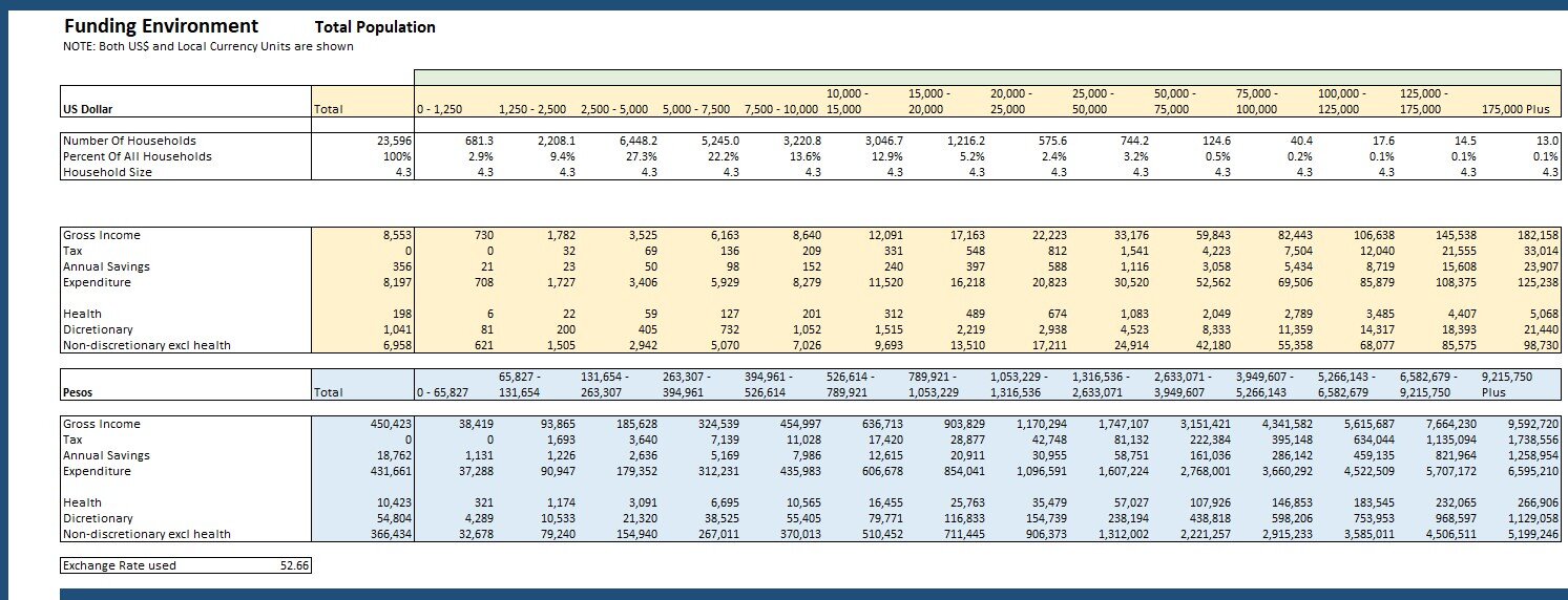
Note: The first table shows both US Dollar and local currency values. For the subsequent two tables the user can switch between either currency at any time. The exchange rate used is shown at the bottom of the first table and is the average rate for 2019.

 

FUNDING SCENARIOS

 

The first part of this section determines

 

• for each year
• at user determined price points
• what proportion of persons with the condition are able to afford to purchase the treatment
• given a user determined funding scenarios.

 

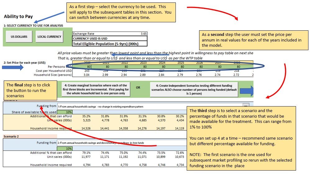
To use this section follow the following steps:

1: Select the currency to be used –

this will apply to all tables in the workbook. – including the distribution of the population by income in the earlier discussed Market Profile Sheet.

 

2: Input the price points

 

This is the price to apply for the treatment for each of the years. Use values appropriate to the selected currency. Also the price entered should be the price to the patient for 1 year.

In this row the user must enter both the first and last year at least (and intervening years if they want) and then by clicking on the button ‘Fill missing values in Price Array’ the intervening points will be filled in using linear trend.

The user can run as many price scenarios as they want. As such you can experiment with multiple price plans.

As all income and expenditure data is expressed in real 2019 values the price points must also be real values. That is, do not factor in inflation (which is impossible to forecast and adds error to forecasts)

 

3: Set up Funding Scenarios

 

How people pay for a treatment varies significantly depending on both the severity of the condition and the cost of the treatment. There are four pre-set scenarios as detailed below – but customised options can be easily added on request.

The model employed here is that the price is compared to the amount of funds available under the selected scenario. If it is below that, then the typical household can afford it. This then identifies the proportion of all persons with the condition that can afford the treatment given that funding scenario. If, for example, it proves to be very small consideration might be given to varying the price or re evaluating the funding scenario used. However, the selected funding scenario should be the one the user feels most closely represents market behaviour.

 

See below for more detail on scenarios

SCENARIOS

There are four pre set funding scenarios as follows

1: From annual savings of the household. This is the 3rd row in the funding section (previous sheet in the workbook). and as shown below. It is in effect surplus funds available to either be saved or cover unusual/unexpected expenditure. Spending from this category means other household expenditure (and lifestyle) does not get disturbed. However, there may be a limit to what proportion of that ‘surplus’ the household is prepared to spend on a (non essential) treatment and the user can define the proportion as well (see below). This is typically used for low cost treatments such as vaccinations.

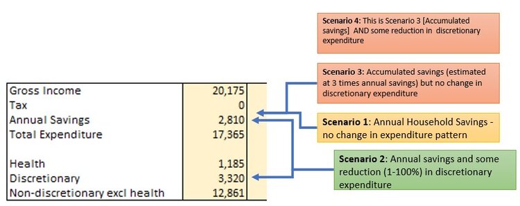
3: From Accumulated Household Savings. Alternatively (and particularly if it is more expensive and important – but perhaps not chronic i.e. a one off hit and the patient is cured) then it may be funded entirely from some or all (user defined) of household accumulated savings rather than disturb the household’s overall living standard/pattern. This is scenario 3 of the pre-set scenarios.

 

4: From Accumulated Savings and Discretionary Expenditure. Finally, if it is expensive and perhaps on going for a period of time it may involve use of accumulated savings and discretionary money. This is typical for treatment of cancers and is scenario 4 of the pre-set scenarios. Again the user can apply a proportion of such funds that the household will so allocate. It would be 100% in the most critical of conditions.

 

COMBINING SCENARIOS

 

Independent Scenarios

This is where each solution is an independent event. This is useful where the user wants to see Price sensitivity. Select one funding scenario for all four scenario boxes and vary the proportion that is used to fund the treatment (e.g. 10% 20% 30% and 40%). This will help the user see what price level will achieve a required volume under different funding scenarios.

Note: In this selection the first scenario is the one used for the ‘Willing to Pay’ Table on the next section.

 

Marginal Scenarios

This is the same as the above expect that it determine what proportion can afford it at the levels set for the 1st scenario, then for the second scenario it excludes – so it shows the marginal gain from moving from scenario 1 to scenario 2 etc. This is useful in that it shows what proportion can afford the treatment at the lowest % input level and then how many resort to a higher percentage etc.

• `

Note: the aggregate reach for all four scenarios is totalled and put at the bottom of this table. It is this data that is used in the ‘Willing to Pay’ sheet on the next page.

 

VACCINE MARKET

This section only appears in the Vaccine Version of the Model (not relevant otherwise)

• `

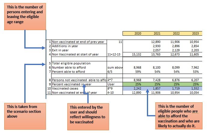
It determines the number of vaccines that would be administered each year from the Non-Vaccinated eligible population given that it can be afforded. NOTE: it assumes 100% willingness to pay.

The user simple enters into the green row the proportion each year of the non-vaccinated population that will get vaccinated in the year. It is to some extent a quick ‘willing to pay’ scenario analysis – ie of those able to pay x% are willing to pay/get vacinated. The next section (Willing to Pay) is a more detailed analysis by income segment and ideally driven by survey data,

PRICE VOLUME VALUE TRADE OFF

 

The third section of Ability to Pay allows the user to see how the price impacts on market size and value under different scenarios in a single year. This is important for the pricing decision. Basically it shows for a selected year how a change in price impacts the total number of people that potentially could afford the treatment and the consequent on market value if all purchased. In short price sensitivity.

Do Note – this stage is determining the maximum market size. Willingness to Pay (the next section ) identifies the proportion of those that can afford the treatment (the market) that will actually purchase.

 

For this section the user

• For this section the user
• selects the year to profile
• selects the funding profile to use
• sets the proportion of that funding scenario that would be available to pay for the treatment (between 1% and 00%)
• sets the minimum price they would be prepared to sell it at and
• a possible maximum price the market would permit.

 

Having determined those parameters press the ‘Run the Scenarios Iterations’ button and the model determines

 

• the proportion of persons with the condition that can afford it
• The number of such persons
• The gross Revenue this generates (price times number of patients who can afford)
• The household income required to be able to afford the treatment under this funding scenario.

 

The chart plots the change in number of patients and total revenue.

GO TO THE NEXT SECTION OF THE MANUAL